| Common normal lines between two shapes 2016.10.20 |
|
|||||||
 Home
HomeChapter: 1. Source code download, 2. Processing method( Newton Raphson ), 3. Test results, 4. Test code,
=> NormalLinesBetweenShapesBasic.zip, NormalLinesBetweenShapes.zip
2. Processing methodreturns=>page top
2.1 Processing steps(Figure 2.1, 2.2)
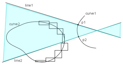
Step1. Test for possible existence of a common normal lines
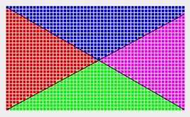
First, divides the curve1 to small segments as shown in Figure 2.1 so as not to have inflection points. Next, creates the normal lines which are line1, line2 at the end points of the small segment. At the same time, divides the curve2 to small segments and cover each small segment by a rectangle (bounding box).
Here, if the all or part of the bounding box which covers the small segment of the curve2 exists in the sandwiched area by the line1 and line2 (light blue area in Figure 2.1), then there is a possibility that the small segment of curve2 and the segment of the curve1 delimitted by p1 and p2 has a common normal line.
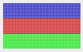
Moreover exchanges the standpoint of curve1 and the curve2 and executes the same test as shown in Figure 2.2, the more accurate possibility for the existence of common normal lines will be given.
Step2. Bisection method to get the higher possibility for the existence of common normal lines
Bisects the couple of segments of the curve1 and curve2 which may have common normal lines and executes the same test described in Step1. Repeats this process by recursive call until the divided segments become enough small.
Step3. High accurate computation by Newton Raphson method
Sets the center points of the enough small segments of the curve1 and curve2 as the initial points and executes the Newton Raphson method.
 |
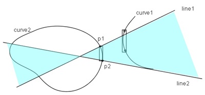 |
| Figure 2.1 Test for possible existence of a common normal lines(1) | Figure 2.2 Test for possible existence of a common normal lines(2) |
2.2 Formulasreturns=>page top
2.2.1 Formulas for Step1 (Figure 2.3(a)-(e))
To test that the all or part of the bounding box exists in the sandwiched area (light blue area in Figure 2.1), it is enough to test whether each of the vertexes of the bounding box is exist in the sandwiched area or not. The following (a)-(d) describes the case that line1 and line2 are not parallel, and the (e) describes the case that they are parallel.
Let e1 and e2 be the unit normal vectors of the line1 and line2 directions, and let ep be the unit vector headed from the point Q to the point p shown as Figure 2.3(a). Here the point Q is the intersection point between the line1 and line2.
We find the condition that the point p exists in the "Region A".
The the outer product between two 2D vectors can be defined in the similar way of that of 3D vectors as follows;
e1×e2 =e1x * e2y - e1y * e2x(1)
Here, the e1×e2 corresponds to z-value of the outer product between two 3D vectors and the e1×e2 represents the signed area of the parallelogram spanned by e1 and e2. Additionally we assume e1×e2≧0 (if not, exchanges e1 and e2).
 :
In the normal cordinate, e1×e2≧0 is satisfied
if the rotation from e1 to e2 is counter clockwise,
however in the graphic coordinate, the outer product≧0 is satisfied if the rotation is clockwise,
because the y-axis is downward.
:
In the normal cordinate, e1×e2≧0 is satisfied
if the rotation from e1 to e2 is counter clockwise,
however in the graphic coordinate, the outer product≧0 is satisfied if the rotation is clockwise,
because the y-axis is downward.(a) The condition that the point p exists in the Region A (Figure 2.3(a)).
0≦e1×ep ≦e1×e2 and 0≦ep×e2 ≦e1×e2(2)
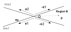
(b) The condition that the point p exists in the Region B (Figure 2.3(b)).
0≦(-e1)×ep≦(-e1)×(-e2) and 0≦ep×(-e2)≦(-e1)×(-e2)
=> -(e1×e2)≦e1×ep≦0 and -(e1×e2)≦ep×e2≦0(3)
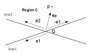
(c) The condition that the point p exists in the Region C (Figure 2.3(c)).
0≦ep×(-e1)≦e2×(-e1) and 0≦e2×ep≦e2×(-e1)
=> 0≦e1×ep≦e1×e2 and 0≦-(ep×e2)≦e1×e2
=> 0≦e1×ep≦e1×e2 and -(e1×e2)≦ep×e2≦0(4)
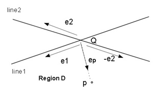
(d) The condition that the point p exists in the Region D (Figure 2.3(d)).
0≦ep×e1≦(-e2)×e1 and 0≦(-e2)×ep≦(-e2)×e1
=> 0≦-(e1×ep)≦e1×e2 and 0≦ep×e2≦e1×e2
=> -(e1×e2)≦e1×ep≦0 and 0 ≦ep×e2≦e1×e2(5)
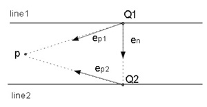
(e) The condition that the point p exists in the sandwitched area between line1 and line2 (Figure 2.3(e)).
Let define the unit vectors: ep1, ep2 and ep shown as Figure 2.3(e), then the condition is following.
0≦en×ep1≦|Q2-Q1| (6)
Here, |Q2-Q1| is the distance between line1 and line2.
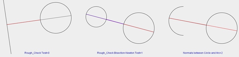
 => The test resuls are shown in Figure 3.1, 3.2.
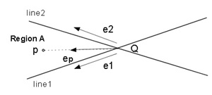 (a) |
 (b) |
 (c) |
 (d) |
 (e) |
|
| Figure 2.3 Formulas for Step1 | |
2.2.2 Newton Raphson method and the formulas for Step3returns=>page top
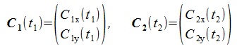
Let t1 and t2 be the parameters of C1 and C2 curves and represents these curves by their x, y components as follows:
Here, bold types represent vectors.
 (1)
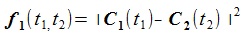
(1)To get a common normal line between two curves, we have to find the t1, t2 which achieve the local minimum of the distance between two curves. The following f1(t1, t2) is the square of the distance bwtween C1 and C2.
 (2)
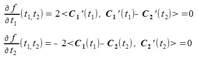
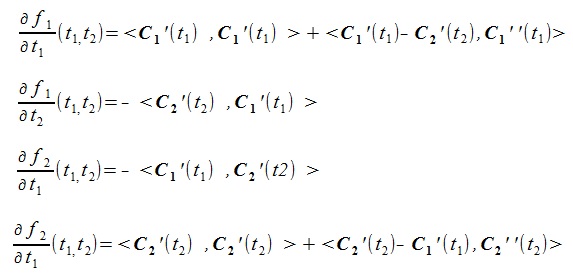
(2)The following conditon is required to minimize the f1(t1, t2) (<a, b> is inner product of vector a and vector b).
 (3)
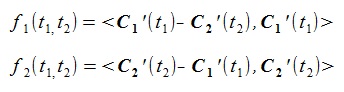
(3)Let f1(t1, t2), f2(t1, t2) be the right side of the abve (3) (ignoring coefficient). then,
 (4)
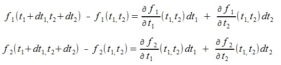
(4)Let dt1, dt2 be very small values or infinitesimals(dt1, dt2 are written as Δt1, Δt2 in a textbook), then the following formulas are derived from the relatons between total differential and partial differential for the f1(t1), t2, f2(t1,t2).
 (5)
(5)Here, the right sides of (5) are represented as follows:
 (6)
(6)The approximation formula of the NewTon-Raphson method is given by setting parts of the left sides of (5) equal 0(zero) as follows.
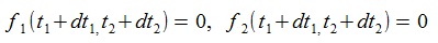 (7)
(7)(5) can be written as follows:
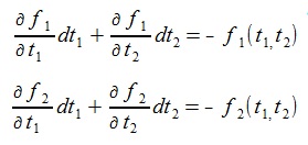 (8)
(8)The matrix representation of (8) is followings:
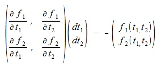 (9)
(9)Let D be the matrix of the left side of (9):
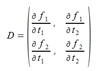 (10)
(10)The dt1, dt2 are given by solving (9) as follows (det means determinant):
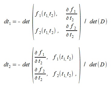 (11)
(11)3. test Resultsreturns=>page top
3.1 Test code: NormalLinesBetweenShapesBasic
|
|
|
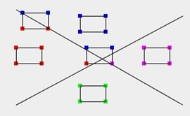
| Figure 3.1(a) The fomulas of Step1(Figure 2.3(a)-(d)) |
Figure 3.1(b) The fomulas of Step1(Figure 2.3(e)) |
Figure 3.1(c) Same as on the left: Display the vertices of the bounding boxes. |
| Display the region code of each vertex by different colors. | ||
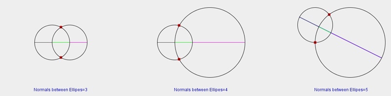
 |
 |
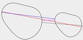 |
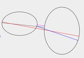
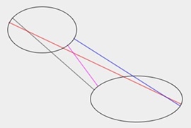
| Figure 3.2(a) ellipse vs. ellipse | Figure 3.2(b) ellipse vs. ellipse | Figure 3.2(c) spline vs. spline |
| Display multiple common normal lines by different colors. | ||
3.2 Test code: NormalLinesBetweenShapes
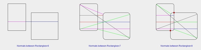
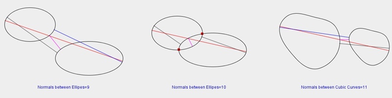
|
Figure 3.3 Computation of various common normal lines(red dots represent intersection points) |
4. Test codereturns=>page top
The code of the NormalLinesBetweenShapes is same as that of NormalLinesBetweenShapesBasic. Only difference is the contents of the Testcases.
4.1 Classes Overview
|
Class |
Description |
|
NormalLinesBetweenShapes |
public class NormalLinesBetweenShapes extends JFrame |
| NormalLinesBetweenShapesPanel |
public class NormalLinesBetweenShapesPanel extends JPanel Draws curves and intersection points on this panel. |
| TestCase |
public class TestCase
=> TestCase of the RegionHitTest.
|
| TestCurve |
public class TestCurve
=> TestCurve of the RegionHitTest.
|
| Parametric Curves |
Segment2D,
Curve2D,
Rectangle2DE,
RoundRectangle2DE,
Ellipse2DE,
Line2DE,
Polyline2DE, CubicCurve2DE, GeneralCurve2DE, FergusonCurve2D |
| Geometric library |
Curve2DUtil.getNormalLinesBetweenShapes,
Curve2DUtil.NormalsInfo subclass, CrossCurvePT, Matrix, Matrix2D |
4.2 Specifications return=>page top
4.2.1 public class NormalLinesBetweenShapesPanel extends JPanel
|
Method |
Description |
| createTestCase |
public void createTestCase() Creates TastCase objects. |
| getGridPoints |
public Point2D[] getGridPoints(Rectangle2D box) parameters: |
| paint |
public void paint(Graphics g) Draws the curves specified by the TestCase objects and the common normal lines on this panel.Calls paintPtRegion, paintRectRegion and paintSolution |
| paintPtRegion |
public void paintPtRegion(Graphics g, TestCase testCase) Processing: =>
Figure 3.1(a), Figure 3.1(b)Formulas=> 2.2.1 Formulas for Step1 |
| paintRectRegion |
public void paintRectRegion(Graphics g, TestCase testCase) 処理: =>
Figure 3.1(c)このクラス(Panel)のオブジェクトにFigure 形と交点を描画する。 paintPtRegion, paintRectRegion, paintSolutionを呼び出す。 |
| paintSolution |
public void paintSolution(Graphics g, TestCase testCase) Processing: =>
Figure 3.2, Figure 3.3Draws common normal lines between two shapes by the Curve2DUtil.getNormalLinesBetweenShapes method. |
All other trademarks are property of their respective owners.